MNIST DNN부터 CNN까지 Deep Learning을 공부함에 있어서 제일 처음으로 접하는 Data는 바로 MNSIT라고 할 수 있습니다. MNIST는 사람들이 직접 필기로 쓴 숫자로써 0부터 9까지 검은 배경에 하얀 글씨로 쓰여져있는 28 x 28 사이즈의 이미지 데이터입니다. 이 포스팅을 통해서 MNIST 데이터를 Deep Learning을 통해서 숫자들을 구별할 수 있는 모델을 설계하고, DNN을 이용한 모델과 CNN을 이용한 모델을 직접 구현해 볼 것입니다.
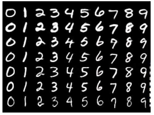
MNSIT 살펴보기 MNIST데이터는 다음 그림과 같은 이미지로 구성되어있습니다.
위에서 설명한 바와 같이 위와 같은 이미지처럼 데이터가 구성되어 있으며, 데이터 하나하나는 다음과 같은 이미지를 구성하고 있습니다.
Deep Learning 모델이 해야할 일은 input으로써 위와 같은 정보를 받고, 해당 데이터가 0부터 9라는 숫자중에 어떤 숫자인지를 알아맞추는 것입니다.
하지만 이 이미지 파일을 어떻게 Deep learning 모델이 받아들일 수 있도록 할 것인가? 보통 MNIST 데이터는 28 x 28의 숫자를 가진 텐서로 표현이 됩니다. 예를 들어서, 하나의 이미지 파일을 텐서로 표현한 데이터를 출력해보면 다음과 같이 나옵니다.
1
2
3
4
5
6
7
8
9
10
11
12
13
14
15
16
17
18
19
20
21
22
23
24
25
26
27
[... 0. 0. 0. 0. 0. 0. 0. 0. 0. 0. 0. 0. 0. 0. 0. 0. 0. 0. 0. 0. 0. 0. 0. 0. 0. 0. 0. 0. 0. 0. 0. 0. 0. 0. 0. 0. 0. 0. 0.01171875 0.0703125 0.0703125 0.0703125 0.4921875 0.53125 0.68359375 0.1015625 0.6484375 0.99609375 0.96484375 0.49609375 0. 0. 0. 0. 0. 0. 0. 0. 0. 0. 0. 0. 0.1171875 0.140625 0.3671875 0.6015625 0.6640625 0.98828125 0.98828125 0.98828125 0.98828125 0.98828125 0.87890625 0.671875 0.98828125 0.9453125 0.76171875 0.25 0. 0. 0. 0. 0. 0. 0. 0. 0. 0. 0. 0.19140625 0.9296875 0.98828125 0.98828125 0.98828125 0.98828125 0.98828125 0.98828125 0.98828125 0.98828125 0.98046875 0.36328125 0.3203125 0.3203125 0.21875 0.15234375 0. 0. 0. 0. 0. 0. 0. 0. 0. 0. 0. 0. 0.0703125 0.85546875 0.98828125 0.98828125 0.98828125 0.98828125 0.98828125 0.7734375 0.7109375 0.96484375 0.94140625 0. 0. 0. 0. 0. 0. 0. 0. 0. 0. 0. 0. 0. 0. 0. 0. 0. 0. 0.3125 0.609375 0.41796875 0.98828125 0.98828125 0.80078125 0.04296875 0. 0.16796875 0.6015 ]
출력된 값 전부를 표현하기에는 너무 많은 숫자들이기에 약간의 데이터만 포스팅하지만, 간단하게 총 784개의 숫자를 가진 데이터임을 확인할 수 있습니다.(28*28=784)
MNIST Practice Pytorch에서 제공하는 기본 MNIST 예제는 CNN으로 이루어져있지만 MNIST는 간단한 데이터이기 때문에, DNN만으로도 충분히 다룰 수 있습니다. 먼저 전체적인 코드를 큰 파트별로 먼저 크게 살펴보고, 그 다음에 하나하나의 파트들을 Line by Line으로 살펴보도록 하겠습니다.
DNN 모델 설계하기 먼저 Pytorch에서 제공하는 라이브러리를 사용하기 위해 각 라이브러리들을 Import 해주는 작업을 해줍니다.
1
2
3
4
5
6
7
8
#Importing Library import torch import torch.nn as nn import torch.nn.functional as F import torch.optim as optim from torchvision import datasets, transforms
그 다음으로는 DNN을 설계를 할 것인데, 우리가 가진 MNIST데이터는 (1,784)의 데이터 형태를 가지고 있고, 구분하려는 숫자의 종류는 총 10가지라는 것을 생각한 뒤 모델을 설계한다고 생각하면 간단한 DNN은 대략 다음과 같이 구성할 수 있습니다.
1
2
3
4
5
6
7
8
9
10
11
12
13
14
15
16
17
18
19
20
21
22
23
24
#Define Neural Networks Model. class Net(nn.Module): def __init__(self): super(Net, self).__init__() self.fc1 = nn.Linear(784, 512) self.fc2 = nn.Linear(512, 256) self.fc3 = nn.Linear(256, 128) self.fc4 = nn.Linear(128, 64) self.fc5 = nn.Linear(64, 32) self.fc6 = nn.Linear(32, 10) def forward(self, x): x = x.float() h1 = F.relu(self.fc1(x.view(-1, 784))) h2 = F.relu(self.fc2(h1)) h3 = F.relu(self.fc3(h2)) h4 = F.relu(self.fc4(h3)) h5 = F.relu(self.fc5(h4)) h6 = self.fc6(h5) return F.log_softmax(h6, dim=1) print("init model done")
여러층의 Feed Forward Network를 설계해서, input size는 784, output size는 10이 되도록 설정해줍니다.(input data는 (1, 784)의 형태이고 정답(숫자의 종류)는 총 10가지)
이 다음에는 DNN을 Training시키기 위해 필요한 여러가지 변수들 및 hyper parameter들을 설정해줍니다.
1 2 3 4 5 6 7 8 9 10 11 12 13 14 15 16 17 18 19 20 batch_size = 64 test_batch_size = 1000 epochs = 10 lr = 0.01 momentum = 0.5 no_cuda = True seed = 1 log_interval = 200 use_cuda = not no_cuda and torch.cuda.is_available() torch.manual_seed(seed) device = torch.device("cuda" if use_cuda else "cpu" ) kwargs = {'num_workers' : 1 , 'pin_memory' : True } if use_cuda else {} print("set vars and device done" )
어느정도 필요한 변수들을 선언해줬다면, 그 다음으로는 pytorch의 torchvision이 제공하는 MNIST 데이터들과 데이터들을 읽어올 수 있는 Loader들을 선언해줍니다.
1 2 3 4 5 6 7 8 9 10 11 12 13 14 15 transform = transforms.Compose([ transforms.ToTensor(), transforms.Normalize((0.1307 ,), (0.3081 ,))]) train_loader = torch.utils.data.DataLoader( datasets.MNIST('../data' , train=True , download=True , transform=transform), batch_size = batch_size, shuffle=True , **kwargs) test_loader = torch.utils.data.DataLoader( datasets.MNIST('../data' , train=False , download=True , transform=transform), batch_size=test_batch_size, shuffle=True , **kwargs)
위와 같이 Data Loader들을 선언해주셨다면, 그 다음으로는 위에서 우리가 설계했던 DNN 모델을 불러오고, Training에 필요한 Optimizer를 선언해줍니다.
1
2
model = Net().to(device) optimizer = optim.SGD(model.parameters(), lr=lr, momentum=momentum)
그 다음으로는 모델을 직접 Training시키는 함수과 Test하는 함수를 구현해줍니다.
1 2 3 4 5 6 7 8 9 10 11 12 13 14 15 16 17 18 19 20 21 22 23 24 25 26 27 28 29 30 31 32 33 def train (log_interval, model, device, train_loader, optimizer, epoch) : model.train() for batch_idx, (data, target) in enumerate(train_loader): data, target = data.to(device), target.to(device) optimizer.zero_grad() output = model(data) loss = F.nll_loss(output, target) loss.backward() optimizer.step() if batch_idx % log_interval == 0 : print('Train Epoch: {} [{}/{} ({:.0f}%)]\tLoss: {:.6f}' .format( epoch, batch_idx * len(data), len(train_loader.dataset), 100. * batch_idx / len(train_loader), loss.item())) def test (log_interval, model, device, test_loader) : model.eval() test_loss = 0 correct = 0 with torch.no_grad(): for data, target in test_loader: data, target = data.to(device), target.to(device) output = model(data) test_loss += F.nll_loss(output, target, reduction='sum' ).item() pred = output.argmax(dim=1 , keepdim=True ) correct += pred.eq(target.view_as(pred)).sum().item() test_loss /= len(test_loader.dataset) print('\nTest set: Average loss: {:.4f}, Accuracy: {}/{} ({:.0f}%)\n' .format (test_loss, correct, len(test_loader.dataset), 100. * correct / len(test_loader.dataset)))
Training Data를 한차례 전부 학습에 사용했다면 그것을 하나의 Epoch이라고 부르는데, 모델을 학습시키는데에 하나의 Epoch보다 더 많은 Epoch이 필요하므로 Train과 Test의 과정을 반복하는 반복문을 선언해줍니다. 이 반복문이 끝나면, 마지막으로 Training된 모델을 저장합니다.
1 2 3 4 5 6 for epoch in range(1 , 11 ): train(log_interval, model, device, train_loader, optimizer, epoch) test(log_interval, model, device, test_loader) torch.save(model, './model.pt' )
여기까지가 Pytorch를 이용해서 DNN으로 MNSIT 데이터들을 분류하는 작업의 코드입니다.
이제는 각 파트별로 소스코드들이 무엇을 의미하는지를 알아보도록 하겠습니다.
DNN Model. 1 2 3 4 5 6 7 8 9 10 11 12 13 14 15 16 17 18 19 class Net(nn.Module): def __init__(self): super(Net, self).__init__() self.fc1 = nn.Linear(784, 512) self.fc2 = nn.Linear(512, 256) self.fc3 = nn.Linear(256, 128) self.fc4 = nn.Linear(128, 64) self.fc5 = nn.Linear(64, 32) self.fc6 = nn.Linear(32, 10) def forward(self, x): x = x.float() h1 = F.relu(self.fc1(x.view(-1, 784))) h2 = F.relu(self.fc2(h1)) h3 = F.relu(self.fc3(h2)) h4 = F.relu(self.fc4(h3)) h5 = F.relu(self.fc5(h4)) h6 = self.fc6(h5) return F.log_softmax(h6, dim=1)
위의 DNN 모델은 총 6개의 Linear 레이어를 통해서 학습하게 됩니다.
MNIST data는 간단한 toy data이고, 간단한 데이터이기 때문에 위처럼
단순한 neural networks만으로도 가능합니다.
784 dimension을 가진 MNIST data를 512, 256, 128, … dimension으로
옮겨가며 feature extraction을 할 수 있도록 하며, 각 레이어마다 끝단에는
Relu라는 activation function을 통해 neural network에 nonlinearity를 추가해줍니다.
마지막 단에 Log Softmax를 통해 마지막 레이어를 지난 10개의 값들을 return하는데
Log Softmax의 역할은 마지막 나온 결과값들을 확률로 취급하여 해석하기 위한 하나의 연산입니다.
Hyper Parameters and Variables 1 2 3 4 5 6 7 8 9 10 11 12 13 14 15 16 17 18 batch_size = 64 test_batch_size = 1000 epochs = 10 lr = 0.01 momentum = 0.5 no_cuda = True seed = 1 log_interval = 200 use_cuda = not no_cuda and torch.cuda.is_available() torch.manual_seed(seed) device = torch.device("cuda" if use_cuda else "cpu" ) kwargs = {'num_workers' : 1 , 'pin_memory' : True } if use_cuda else {} print("set vars and device done" )
위의 parameter들은 보통 딥러닝 모델을 train할 때, 많이 쓰이는 변수들이며
딥러닝 모델에 큰 영향을 주는 parameter는 hyper parameter라고 합니다.
batch_size란, cpu 혹은 gpu에 한번에 몇개씩의 data를 넣어줄 것인지를 정하는 것입니다.
batch_size의 갯수에 따라서도 딥러닝 모델의 성능이 크게 달라집니다.
epochs같은 경우에는 training data를 1번씩 모두 썼을 때까지를 1 epoch이 지났다고 합니다.
즉, training data가 10개가 있고, 그 data들을 모두 한번씩 training에 썼다면, 1 epoch이 지난 것입니다.
Data Loader 1 2 3 4 5 6 7 8 9 10 11 12 13 14 15 transform = transforms.Compose([ transforms.ToTensor(), transforms.Normalize((0.1307 ,), (0.3081 ,))]) train_loader = torch.utils.data.DataLoader( datasets.MNIST('../data' , train=True , download=True , transform=transform), batch_size = batch_size, shuffle=True , **kwargs) test_loader = torch.utils.data.DataLoader( datasets.MNIST('../data' , train=False , download=True , transform=transform), batch_size=test_batch_size, shuffle=True , **kwargs)
transform을 통해서 data를 어떻게 처리해줄지 결정을 해줍니다.
함수를 보면, 이미지 데이터를 .ToTensor()를 통해서 tensor형태로 데이터를 변환해준 뒤
Normalize과정을 해주기 위해서 standard deviation와 variation 값을 직접 입력해줍니다. (모든 MNIST이미지를 통해 미리 구해놓은 값입니다.)
그리고 위의 함수에 따라 training set과 test set을 구분해서 만들어줍니다.
현재 torchvision의 함수 자체가 ‘train’이라는 parameter를 통해 training set과 test set을 쉽게 준비할 수 있도록 설계해놨기 때문에, 이를 그대로 사용하시면 됩니다.
Optimizer 1 2 model = Net().to(device) optimizer = optim.SGD(model.parameters(), lr=lr, momentum=momentum)
Optimizer를 통해서 모델이 어떤 방식으로 training할지를 고르게 됩니다.
대표적인 training방식은 SGD, RMSprop, Adam, AdaDelta 등 여러가지 방식이 있는데
위의 코드는 SGD와 momentum을 사용하는 optimizer를 설정해준 뒤, model내의 parameter들을 training하도록 했습니다.
Train and Test 1 2 3 4 5 6 7 8 9 10 11 12 13 14 15 16 17 18 19 20 21 22 23 24 25 26 27 28 29 30 31 32 33 def train (log_interval, model, device, train_loader, optimizer, epoch) : model.train() for batch_idx, (data, target) in enumerate(train_loader): data, target = data.to(device), target.to(device) optimizer.zero_grad() output = model(data) loss = F.nll_loss(output, target) loss.backward() optimizer.step() if batch_idx % log_interval == 0 : print('Train Epoch: {} [{}/{} ({:.0f}%)]\tLoss: {:.6f}' .format( epoch, batch_idx * len(data), len(train_loader.dataset), 100. * batch_idx / len(train_loader), loss.item())) def test (log_interval, model, device, test_loader) : model.eval() test_loss = 0 correct = 0 with torch.no_grad(): for data, target in test_loader: data, target = data.to(device), target.to(device) output = model(data) test_loss += F.nll_loss(output, target, reduction='sum' ).item() pred = output.argmax(dim=1 , keepdim=True ) correct += pred.eq(target.view_as(pred)).sum().item() test_loss /= len(test_loader.dataset) print('\nTest set: Average loss: {:.4f}, Accuracy: {}/{} ({:.0f}%)\n' .format (test_loss, correct, len(test_loader.dataset), 100. * correct / len(test_loader.dataset)))
train함수를 통해서 train data들을 한번씩 살피도록 합니다.
test함수를 통해서 test data를 통해 모델의 성능을 평가하게 됩니다.
Make machine works 1 2 3 4 5 6 for epoch in range(1 , 11 ): train(log_interval, model, device, train_loader, optimizer, epoch) test(log_interval, model, device, test_loader) torch.save(model, './model.pt' )
train 함수와 test함수를 통해 model을 트레이닝 시키고
CNN model CNN 모델은 28x28의 MNIST data를 1x784로 고쳐서 쓰는 것이 아닌, 2d data의 형태 그대로 사용하게 됩니다.
1 2 3 4 5 6 7 8 9 10 11 12 13 14 15 16 17 18 19 20 21 22 23 24 class Net (nn.Module) : def __init__ (self) : super(Net, self).__init__() self.conv1 = nn.Conv2d(1 , 32 , 3 , 1 ) self.conv2 = nn.Conv2d(32 , 64 , 3 , 1 ) self.dropout1 = nn.Dropout2d(0.25 ) self.dropout2 = nn.Dropout2d(0.5 ) self.fc1 = nn.Linear(9216 , 128 ) self.fc2 = nn.Linear(128 , 10 ) def forward (self, x) : x = self.conv1(x) x = F.relu(x) x = self.conv2(x) x = F.relu(x) x = F.max_pool2d(x, 2 ) x = self.dropout1(x) x = torch.flatten(x, 1 ) x = self.fc1(x) x = F.relu(x) x = self.dropout2(x) x = self.fc2(x) output = F.log_softmax(x, dim=1 ) return output
CNN을 이해하기 위해서는 filter size, padding, stride 라는 개념을 알아두셔야 합니다.